Overview
speedyBBT is an R package for fitting Bradley-Terry models to pairwise comparison data using fast, fully Bayesian MCMC. Given a set of pairwise judgements – which of two wards has the higher rate of forced marriage, which of two tennis players won a match, which of two neighbourhoods looks more deprived – speedyBBT estimates a quality parameter for every item being compared, along with full posterior uncertainty.
Inference is carried out using a Pólya-Gamma data augmentation scheme, which makes sampling fast even for large numbers of items and comparisons. The package supports:
- the standard Bradley-Terry model (
speedyBBTm()), optimised for speed when there are no ties or comparison-specific effects; - ties, comparison-specific effects (e.g. home advantage), and item-level covariates via a formula interface (
BBTm()); - multivariate normal prior distributions on the item quality parameters, so that structure between items (e.g. spatial adjacency) can be encoded directly into the prior;
- optional hyperparameter inference on the prior scale.
The package can be used with data collected using the Comparative Judgement Interface.
Getting started
If you’re new to speedyBBT, start with the Getting started with speedyBBT vignette, which walks through fitting a model to real comparative-judgement data end to end.
Installation
Install the released version from CRAN:
install.packages("speedyBBT")
# for development version
# devtools::install_github("rowlandseymour/speedyBBT", dependencies = TRUE)
Usage
The code chunks below show how to use the package to fit the Bradley–Terry model to a data set relating to forced marriage. Judges were shown pairs of wards and asked which had a higher rate of forced marriage. We can use the speedyBBTm function to draw samples for the full conditional distributions for the ward quality parameters. We place a multivariate normal prior distribution on the ward quality parameters. The covariance matrix of this prior distribution is constructed using a network representation of the wards in Nottinghamshire.
# View Data
data("forcedMarriage", package = "speedyBBT")
head(forcedMarriage$comparisons)
#>   user            time win lost
#> 1    1 16:08:26.316839  67   31
#> 2    1 16:08:47.888894  19    9
#> 3    1 16:09:14.093517  18   74
#> 4    1 16:09:23.666987  56   68
#> 5    1 16:09:42.930976  50   66
#> 6    1 16:09:51.129570  53   15


# Construct covariance matrix
expA <- expm::expm(forcedMarriage$adjacencyMatrix)
prior.var <- diag(diag(expA)^-0.5) %*% expA %*% diag(diag(expA)^-0.5)

# Fit model
library(speedyBBT)
forcedMarriageModel <- speedyBBTm(
  outcome = rep(1, length(forcedMarriage$comparisons$win)),
  player1 = forcedMarriage$comparisons$win,
  player2 = forcedMarriage$comparisons$lost,
  player.prior.var = prior.var
)
lambda_draws <- parameter(forcedMarriageModel, "lambda")
lambda_centered <- lambda_draws - rowMeans(lambda_draws)

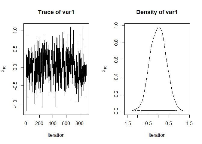
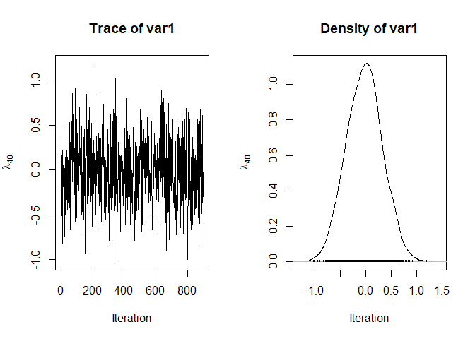
# View Trace Plots
plot(lambda_centered[, 10],
  type = "l",
  xlab = "Iteration", ylab = expression(lambda[10])
)
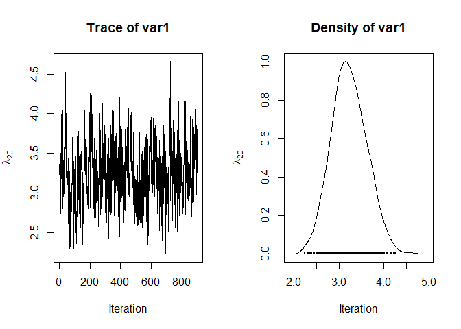
plot(lambda_centered[, 20],
  type = "l",
  xlab = "Iteration", ylab = expression(lambda[20])
)
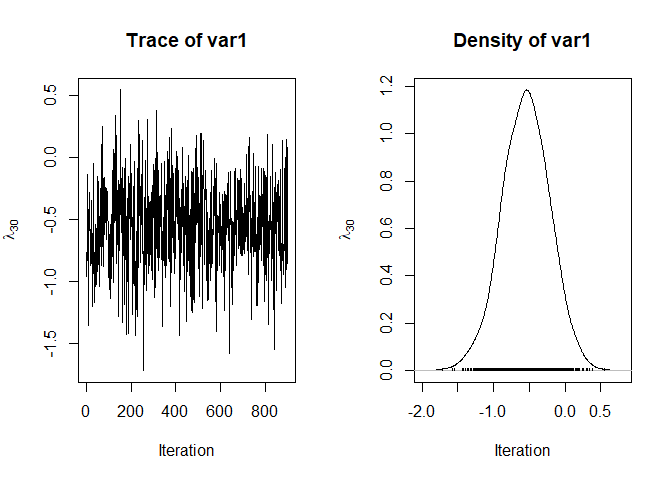
plot(lambda_centered[, 30],
  type = "l",
  xlab = "Iteration", ylab = expression(lambda[30])
)
plot(lambda_centered[, 40],
  type = "l",
  xlab = "Iteration", ylab = expression(lambda[40])
)
# View Results
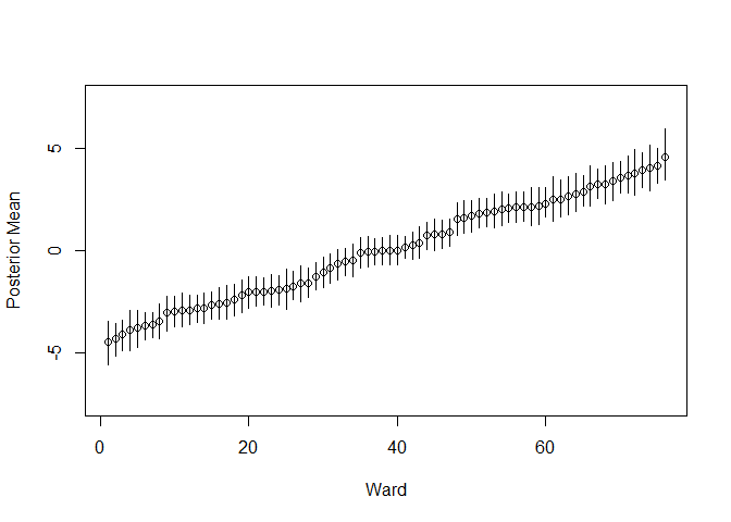
forcedMarriageModelMeans <- colMeans(lambda_draws)
forcedMarriageModelLowerCI <- apply(lambda_draws, 2, quantile, 0.025)
forcedMarriageModelUpperCI <- apply(lambda_draws, 2, quantile, 0.975)
forcedMarriageResults <- data.frame(
  "ward" = forcedMarriage$wards$NAME,
  "mean" = forcedMarriageModelMeans,
  "lowerCI" = forcedMarriageModelLowerCI,
  "upperCI" = forcedMarriageModelUpperCI
)
forcedMarriageResults <- forcedMarriageResults[order(forcedMarriageResults$mean), ]

plot(forcedMarriageResults$mean, xlab = "Ward", ylab = "Posterior Mean", ylim = c(-7.5, 7.5))
segments(
  x0 = 1:nrow(forcedMarriageResults), y0 = forcedMarriageResults$lowerCI,
  y1 = forcedMarriageResults$upperCI
)
References
- J. Jiang, J. Marsh, and R. G. Seymour. 2026. A reduced basis decomposition approach to efficient data collection in pairwise comparison studies. Computational Statistics.
- R. G. Seymour, A. Nyarko-Agyei, H. R. McCabe,K. Severn,D.Sirl, T. Kypraios, A. Taylor. 2025. Comparative Judgement Modeling to Map Forced Marriage at Local Levels. Annals of Applied Statistics.
- R. G. Seymour, D. Sirl, S. Preston, and J. Goulding. 2023. Multi-Level Spatial Comparative Judgement Models to Map Deprivation. Proceedings of the Joint Statistical Meeting 2023.
- R. G. Seymour, D. Sirl, S. Preston,|. L. Dryden, B. Perrat, M. J. A. Ellis, and J. Goulding. 2022. The Bayesian Spatial Bradley-Terry model: Urban deprivation modelling in Tanzania. Journal of the Royal Statistical Society: C. 71 (2).
Acknowledgements
This work is supported by a UKRI Future Leaders Fellowship [MR/X034992/1].
Previously, it has been supported by the Engineering and Physical Sciences Research Council [grant numbers EP/T003928/1, EP/R513283/1], the Economic and Social Sciences Research Council [ES/V015370/1] and the Research England Policy Support Fund.
The Dar es Salaam comparative judgement dataset was collected by Madeleine Ellis, James Goulding, Bertrand Perrat, Gavin Smith and Gregor Engelmann. We gratefully acknowledge the Rights Lab at the University of Nottingham for supporting funding for the comprehensive ground truth survey. We also acknowledge Humanitarian Street Mapping Team (HOT) for providing a team of experts in data collection to facilitate the surveys. This fieldwork was also supported by the EPSRC Horizon Centre for Doctoral Training - My Life in Data (EP/L015463/1) and by EPSRC grant Neodemographics (EP/L021080/1).
The data in Nottinghamshire was collected with support from the Nottinghamshire Slavery Multi Agency Risk Assessment Conference. Data in South Yorkshire was collected with support from South Yorkshire Police. Data in Wokingham was collected with support from Wokingham Council. Data in Oxfordshire was collected with support from Oxford Against Cutting. Data in West Yorkshire was collected with support from West Yorkshire Police and Karma Nirvana.