speedyBBT is a package for Bayesian Bradley-Terry
modelling. It provides functions for fitting the Bradley-Terry model
using Markov Chain Monte Carlo (MCMC) methods, allowing for inference on
player abilities and hyperparameters. It uses latent Pólya-Gamma
variables to facilitate efficient sampling.
To fit a Bradley-Terry model using speedyBBT, you can
first install the package from CRAN or install the development version
from GitHub.
# Install from CRAN
# install.packages("speedyBBT")
# Install the development version from GitHub
# remotes::install_github("rowlandseymour/speedyBBT")
You can learn more about the package functions and how to use them
from the documentation which can be accessed using
?function_name in R. For example, to learn about the
speedyBBTm function, you can run:
?speedyBBTmThe package includes some example datasets that you can use to
practice fitting models. These datasets are automatically loaded when
you install the package. To view the forcedMarriage
dataset, you can run:
data("forcedMarriage")This dataset was collected from 12 judges in Nottinghamshire who were asked to judge which of a pair of 76 wards had a higher risk of forced marriage. The dataset contains the results of the 1,846 pairwise comparisons made by the judges. An adjacency matrix is constructed based on proximity, assuming that geographically close wards are more highly correlated. This serves as a covariance matrix for the multivariate normal prior distribution of the item qualities. In this case, the “items” are wards in Nottinghamshire and their “quality” is the risk of forced marriage in that ward.
The speedyBBTm function can be used to fit a
Bradley-Terry model to the data. To start with, you need to construct
the prior distribution for the item qualities. This needs to be a Normal
distribution. For this example, you can use the adjacency matrix
provided with the package data and then use it to create a covariance
matrix for the prior distribution of the item qualities. For your own
data set, you will want to create an adjacency matrix with values that
denote the similarity of different items to one another. For this
example, the adjacency matrix ranks wards that are closer to one another
as more similar. You can specify the outcome variable, the items
involved in each comparison, and any prior information you have about
the items’ rating. In this example, the items are the individual wards.
The function will return an MCMC object containing samples from the
posterior distribution of the item qualities.
# Construct covariance matrix
expA <- expm::expm(forcedMarriage$adjacencyMatrix)
prior.var <- diag(diag(expA)^-0.5) %*% expA %*% diag(diag(expA)^-0.5)
Next, you can fit the model using the speedyBBTm()
function. You will need to specify the outcome variable, the items
involved in each comparison, and the prior covariance matrix for the
item qualities. You can also specify the number of MCMC iterations to
run. This example uses the default values for the hyperparameters of the
prior distribution, but you can also specify your own values if you have
prior knowledge about the items’ rating using the
hyperparameter argument. To match the plots in this
vignette, you will need to use the same argument to
set.seed as the one provided here.
# Fit model
set.seed(432)
forcedMarriageModel <- speedyBBTm(
  outcome = rep(1, length(forcedMarriage$comparisons$win)),
  player1 = forcedMarriage$comparisons$win,
  player2 = forcedMarriage$comparisons$lost,
  player.prior.var = prior.var,
  n.iter = 1000,
  burn.in = 100
)
To view some preliminary information about the results, you can calculate the means of the item quality parameters from the MCMC samples and summarise them. This will give you an idea of the estimated qualities of the items based on the comparisons in the dataset.
forcedMarriageModelMeans <- colMeans(forcedMarriageModel[, grep("lambda", varnames(forcedMarriageModel))])
forcedMarriageModelMeans
#>    lambda[1]    lambda[2]    lambda[3]    lambda[4]    lambda[5]    lambda[6]
#>  4.537826683  1.908970996  2.682688993  2.139152409  3.859816397  3.594924822
#>    lambda[7]    lambda[8]    lambda[9]   lambda[10]   lambda[11]   lambda[12]
#>  3.334383929  4.061449956 -0.065205764  0.053868794  1.694547168  1.546731278
#>   lambda[13]   lambda[14]   lambda[15]   lambda[16]   lambda[17]   lambda[18]
#>  0.790469378  0.202785405  1.989669905 -0.047192195 -0.664364241  2.140416409
#>   lambda[19]   lambda[20]   lambda[21]   lambda[22]   lambda[23]   lambda[24]
#>  2.819732086  3.203223587  1.567280463  2.267801012  0.030311219  2.027193465
#>   lambda[25]   lambda[26]   lambda[27]   lambda[28]   lambda[29]   lambda[30]
#>  3.936813693  2.102001555  3.143541786 -0.056488774 -1.205794549 -0.511368520
#>   lambda[31]   lambda[32]   lambda[33]   lambda[34]   lambda[35]   lambda[36]
#> -0.826200918  3.711550263  0.738504066  0.390084333  0.811664588  0.874172292
#>   lambda[37]   lambda[38]   lambda[39]   lambda[40]   lambda[41]   lambda[42]
#>  2.478825810 -0.497859197  0.231883090 -0.005764598  2.737133969  2.393091021
#>   lambda[43]   lambda[44]   lambda[45]   lambda[46]   lambda[47]   lambda[48]
#>  2.227799936  3.528443134  3.157938997 -2.486823424 -1.971053615 -3.037149271
#>   lambda[49]   lambda[50]   lambda[51]   lambda[52]   lambda[53]   lambda[54]
#> -2.094810491  1.839431812 -1.645926980 -1.789073819 -1.577046906 -2.009310458
#>   lambda[55]   lambda[56]   lambda[57]   lambda[58]   lambda[59]   lambda[60]
#>  1.866008315 -2.933034133 -1.986600458 -1.742389548 -3.636681473 -3.476970328
#>   lambda[61]   lambda[62]   lambda[63]   lambda[64]   lambda[65]   lambda[66]
#> -1.902973910 -2.580509197 -2.941464501 -2.827955667 -3.643306289 -3.878715107
#>   lambda[67]   lambda[68]   lambda[69]   lambda[70]   lambda[71]   lambda[72]
#> -2.668409294 -4.123388153 -1.936405667 -4.491188312 -2.951354245 -4.312123789
#>   lambda[73]   lambda[74]   lambda[75]   lambda[76]
#> -2.838690691 -2.439364544 -3.799817125 -1.019356865
summary(forcedMarriageModel)
#>
#> Iterations = 1:900
#> Thinning interval = 1
#> Number of chains = 1
#> Sample size per chain = 900
#>
#> 1. Empirical mean and standard deviation for each variable,
#>    plus standard error of the mean:
#>
#>                 Mean     SD Naive SE Time-series SE
#> lambda[1]   4.537827 0.5917 0.019724        0.03600
#> lambda[2]   1.908971 0.4257 0.014189        0.03130
#> lambda[3]   2.682689 0.4723 0.015744        0.02555
#> lambda[4]   2.139152 0.4539 0.015130        0.02629
#> lambda[5]   3.859816 0.4349 0.014496        0.02351
#> lambda[6]   3.594925 0.4125 0.013750        0.02625
#> lambda[7]   3.334384 0.4319 0.014395        0.02479
#> lambda[8]   4.061450 0.4533 0.015108        0.02701
#> lambda[9]  -0.065206 0.3743 0.012478        0.01792
#> lambda[10]  0.053869 0.3704 0.012346        0.01834
#> lambda[11]  1.694547 0.3661 0.012202        0.01792
#> lambda[12]  1.546731 0.3656 0.012188        0.01785
#> lambda[13]  0.790469 0.3549 0.011831        0.01800
#> lambda[14]  0.202785 0.2795 0.009317        0.01345
#> lambda[15]  1.989670 0.4094 0.013648        0.02752
#> lambda[16] -0.047192 0.3129 0.010431        0.01291
#> lambda[17] -0.664364 0.3638 0.012127        0.02230
#> lambda[18]  2.140416 0.3652 0.012173        0.02065
#> lambda[19]  2.819732 0.4022 0.013406        0.02484
#> lambda[20]  3.203224 0.3719 0.012398        0.02250
#> lambda[21]  1.567280 0.4211 0.014036        0.02079
#> lambda[22]  2.267801 0.3560 0.011866        0.02054
#> lambda[23]  0.030311 0.3579 0.011929        0.01726
#> lambda[24]  2.027193 0.3581 0.011938        0.02114
#> lambda[25]  3.936814 0.5549 0.018495        0.04016
#> lambda[26]  2.102002 0.3742 0.012474        0.01822
#> lambda[27]  3.143542 0.4184 0.013947        0.02140
#> lambda[28] -0.056489 0.3573 0.011910        0.01857
#> lambda[29] -1.205795 0.3375 0.011251        0.01876
#> lambda[30] -0.511369 0.3299 0.010997        0.01650
#> lambda[31] -0.826201 0.3688 0.012294        0.01677
#> lambda[32]  3.711550 0.5507 0.018356        0.03570
#> lambda[33]  0.738504 0.3430 0.011435        0.01590
#> lambda[34]  0.390084 0.4269 0.014229        0.02138
#> lambda[35]  0.811665 0.3764 0.012547        0.01965
#> lambda[36]  0.874172 0.3186 0.010620        0.01411
#> lambda[37]  2.478826 0.4330 0.014434        0.02213
#> lambda[38] -0.497859 0.3992 0.013308        0.02116
#> lambda[39]  0.231883 0.3746 0.012486        0.01819
#> lambda[40] -0.005765 0.3630 0.012099        0.02017
#> lambda[41]  2.737134 0.4590 0.015299        0.02628
#> lambda[42]  2.393091 0.5979 0.019929        0.03680
#> lambda[43]  2.227800 0.4771 0.015903        0.02663
#> lambda[44]  3.528443 0.3984 0.013281        0.02176
#> lambda[45]  3.157939 0.4902 0.016339        0.02812
#> lambda[46] -2.486823 0.4549 0.015164        0.03235
#> lambda[47] -1.971054 0.3490 0.011634        0.01712
#> lambda[48] -3.037149 0.3929 0.013096        0.02281
#> lambda[49] -2.094810 0.3877 0.012923        0.02709
#> lambda[50]  1.839432 0.3738 0.012459        0.01699
#> lambda[51] -1.645927 0.4370 0.014567        0.02097
#> lambda[52] -1.789074 0.4821 0.016069        0.02329
#> lambda[53] -1.577047 0.3790 0.012634        0.02118
#> lambda[54] -2.009310 0.3888 0.012959        0.02463
#> lambda[55]  1.866008 0.3477 0.011589        0.02086
#> lambda[56] -2.933034 0.4106 0.013688        0.02110
#> lambda[57] -1.986600 0.3422 0.011406        0.01624
#> lambda[58] -1.742390 0.3251 0.010837        0.01520
#> lambda[59] -3.636681 0.3370 0.011234        0.02249
#> lambda[60] -3.476970 0.4581 0.015271        0.03139
#> lambda[61] -1.902974 0.3505 0.011682        0.01704
#> lambda[62] -2.580509 0.3922 0.013073        0.02064
#> lambda[63] -2.941465 0.3788 0.012626        0.02235
#> lambda[64] -2.827956 0.3269 0.010895        0.01989
#> lambda[65] -3.643306 0.3325 0.011082        0.02545
#> lambda[66] -3.878715 0.4921 0.016403        0.03375
#> lambda[67] -2.668409 0.3429 0.011429        0.01861
#> lambda[68] -4.123388 0.4000 0.013332        0.02363
#> lambda[69] -1.936406 0.4003 0.013342        0.01937
#> lambda[70] -4.491188 0.5769 0.019231        0.03856
#> lambda[71] -2.951354 0.4338 0.014462        0.03015
#> lambda[72] -4.312124 0.4197 0.013989        0.02978
#> lambda[73] -2.838691 0.3878 0.012927        0.02161
#> lambda[74] -2.439365 0.3930 0.013101        0.02149
#> lambda[75] -3.799817 0.4317 0.014392        0.02454
#> lambda[76] -1.019357 0.4000 0.013332        0.02085
#> alpha.sq   12.944356 4.7604 0.158680        0.47716
#>
#> 2. Quantiles for each variable:
#>
#>                2.5%       25%       50%     75%    97.5%
#> lambda[1]   3.51087  4.117670  4.505731  4.9181  5.87871
#> lambda[2]   1.08757  1.637768  1.911995  2.1806  2.72540
#> lambda[3]   1.80571  2.363719  2.657650  2.9738  3.68534
#> lambda[4]   1.26815  1.826677  2.149424  2.4292  3.02973
#> lambda[5]   2.99281  3.567111  3.836172  4.1500  4.71556
#> lambda[6]   2.84945  3.308206  3.578396  3.8803  4.44080
#> lambda[7]   2.54224  3.040079  3.331775  3.6289  4.20693
#> lambda[8]   3.20659  3.762512  4.052154  4.3507  4.98445
#> lambda[9]  -0.80844 -0.321772 -0.069996  0.1661  0.65731
#> lambda[10] -0.64234 -0.189172  0.026260  0.3091  0.83908
#> lambda[11]  1.02723  1.436115  1.690030  1.9315  2.40541
#> lambda[12]  0.84585  1.297454  1.545794  1.7749  2.30823
#> lambda[13]  0.14725  0.563772  0.811474  1.0132  1.46442
#> lambda[14] -0.34456  0.021564  0.203841  0.3870  0.75963
#> lambda[15]  1.26265  1.704473  1.966004  2.2596  2.83630
#> lambda[16] -0.63897 -0.271685 -0.048850  0.1521  0.58279
#> lambda[17] -1.40571 -0.904387 -0.658031 -0.4187  0.05043
#> lambda[18]  1.44585  1.890907  2.141286  2.3978  2.82835
#> lambda[19]  2.06696  2.547058  2.806786  3.0863  3.63256
#> lambda[20]  2.47808  2.962840  3.194907  3.4615  3.92845
#> lambda[21]  0.73126  1.269948  1.574273  1.8432  2.40216
#> lambda[22]  1.61608  2.003842  2.269554  2.5096  3.01341
#> lambda[23] -0.65149 -0.218892  0.020986  0.2794  0.72037
#> lambda[24]  1.31394  1.784942  2.027934  2.2546  2.73095
#> lambda[25]  2.87898  3.551824  3.926525  4.3103  5.02771
#> lambda[26]  1.34805  1.858209  2.112523  2.3538  2.82862
#> lambda[27]  2.35669  2.848758  3.149104  3.4234  3.99822
#> lambda[28] -0.74414 -0.290266 -0.063552  0.1868  0.64244
#> lambda[29] -1.87497 -1.432475 -1.202108 -0.9860 -0.52591
#> lambda[30] -1.17921 -0.734171 -0.500735 -0.2821  0.12316
#> lambda[31] -1.53776 -1.071670 -0.819482 -0.5815 -0.09886
#> lambda[32]  2.67797  3.310853  3.702028  4.0672  4.83869
#> lambda[33]  0.03314  0.505285  0.741048  0.9714  1.37956
#> lambda[34] -0.42023  0.085915  0.386847  0.6866  1.19528
#> lambda[35]  0.06722  0.553817  0.812627  1.0622  1.53288
#> lambda[36]  0.26374  0.662811  0.884501  1.0886  1.51049
#> lambda[37]  1.65730  2.181019  2.467786  2.7509  3.40670
#> lambda[38] -1.26271 -0.764560 -0.497277 -0.2324  0.28917
#> lambda[39] -0.51211 -0.009278  0.230008  0.4770  0.95758
#> lambda[40] -0.74022 -0.256494  0.005077  0.2441  0.72219
#> lambda[41]  1.89543  2.411363  2.706810  3.0248  3.67469
#> lambda[42]  1.29694  1.991420  2.357005  2.7746  3.66514
#> lambda[43]  1.32974  1.908589  2.221755  2.5406  3.18759
#> lambda[44]  2.74675  3.259063  3.513751  3.7828  4.33203
#> lambda[45]  2.21529  2.822364  3.141748  3.4957  4.12458
#> lambda[46] -3.44891 -2.787834 -2.468651 -2.1696 -1.58830
#> lambda[47] -2.68950 -2.204860 -1.969589 -1.7388 -1.30111
#> lambda[48] -3.87765 -3.299676 -3.027878 -2.7803 -2.26407
#> lambda[49] -2.92694 -2.343746 -2.087916 -1.8439 -1.33426
#> lambda[50]  1.15177  1.596613  1.833008  2.0765  2.60947
#> lambda[51] -2.55697 -1.930073 -1.618603 -1.3492 -0.80264
#> lambda[52] -2.80499 -2.113574 -1.768475 -1.4464 -0.92800
#> lambda[53] -2.34585 -1.810430 -1.574650 -1.3217 -0.84567
#> lambda[54] -2.84274 -2.261285 -1.994941 -1.7284 -1.29825
#> lambda[55]  1.14970  1.638351  1.876254  2.0812  2.53968
#> lambda[56] -3.74619 -3.196562 -2.934224 -2.6550 -2.20477
#> lambda[57] -2.64978 -2.204936 -1.990924 -1.7464 -1.31070
#> lambda[58] -2.35940 -1.971113 -1.756006 -1.5098 -1.09418
#> lambda[59] -4.29590 -3.865121 -3.631374 -3.4004 -3.01670
#> lambda[60] -4.32507 -3.774993 -3.491695 -3.1904 -2.55288
#> lambda[61] -2.59143 -2.134782 -1.912216 -1.6642 -1.20751
#> lambda[62] -3.37661 -2.839194 -2.565677 -2.2936 -1.85991
#> lambda[63] -3.71519 -3.186004 -2.939253 -2.6925 -2.21287
#> lambda[64] -3.48345 -3.039564 -2.823733 -2.6028 -2.20127
#> lambda[65] -4.32500 -3.854074 -3.638345 -3.4184 -3.03776
#> lambda[66] -4.84364 -4.198529 -3.879378 -3.5603 -2.91777
#> lambda[67] -3.37416 -2.896275 -2.652161 -2.4387 -2.00756
#> lambda[68] -4.91573 -4.395995 -4.119695 -3.8425 -3.35079
#> lambda[69] -2.69684 -2.215454 -1.933209 -1.6903 -1.17628
#> lambda[70] -5.70185 -4.828699 -4.471539 -4.0761 -3.50908
#> lambda[71] -3.79821 -3.240908 -2.964309 -2.6457 -2.09841
#> lambda[72] -5.19560 -4.581842 -4.294365 -4.0293 -3.52285
#> lambda[73] -3.62383 -3.077175 -2.853230 -2.5712 -2.12108
#> lambda[74] -3.19234 -2.696463 -2.450547 -2.1614 -1.66898
#> lambda[75] -4.69040 -4.085319 -3.793155 -3.5017 -3.00282
#> lambda[76] -1.82654 -1.288954 -1.012126 -0.7398 -0.24574
#> alpha.sq    6.04358  9.729142 12.042500 15.3454 24.25715
You can run some MCMC diagnostics to check convergence. The
speedyBBTm() function returns an “mcmc” object that
can be used with the coda package for diagnostics. You can
use the effectiveSize() function to calculate the estimated
effective sample size for convergence. Another example diagnostic
illustrated here is the Geweke diagnostic, calculated using the
gewecke.diag() function from coda. This
diagnostic compares the difference between the two sample means in the
first 10% and the last 50% of iterations in the Markov chain to assess
convergence. For more information about available plots and diagnostics,
you can refer to the coda
package documentation.
effectiveSize(forcedMarriageModel)
#>  lambda[1]  lambda[2]  lambda[3]  lambda[4]  lambda[5]  lambda[6]  lambda[7]
#>  270.12368  184.94687  341.72287  298.00677  342.05023  246.97676  303.53240
#>  lambda[8]  lambda[9] lambda[10] lambda[11] lambda[12] lambda[13] lambda[14]
#>  281.60246  436.20370  408.06923  417.41677  419.39075  388.79301  432.05236
#> lambda[15] lambda[16] lambda[17] lambda[18] lambda[19] lambda[20] lambda[21]
#>  221.26773  587.12814  266.21247  312.87282  262.10651  273.35051  410.04084
#> lambda[22] lambda[23] lambda[24] lambda[25] lambda[26] lambda[27] lambda[28]
#>  300.26353  429.93178  287.09694  190.86499  421.64829  382.23555  370.35245
#> lambda[29] lambda[30] lambda[31] lambda[32] lambda[33] lambda[34] lambda[35]
#>  323.87058  399.63964  483.52430  237.98391  465.49248  398.64729  366.92161
#> lambda[36] lambda[37] lambda[38] lambda[39] lambda[40] lambda[41] lambda[42]
#>  509.54264  383.03690  355.92071  424.07792  323.98088  305.04277  264.00841
#> lambda[43] lambda[44] lambda[45] lambda[46] lambda[47] lambda[48] lambda[49]
#>  321.03627  335.24133  303.85557  197.70550  415.53381  296.66142  204.82436
#> lambda[50] lambda[51] lambda[52] lambda[53] lambda[54] lambda[55] lambda[56]
#>  484.06170  434.32532  428.32838  320.22810  249.11390  277.86443  378.84002
#> lambda[57] lambda[58] lambda[59] lambda[60] lambda[61] lambda[62] lambda[63]
#>  443.77081  457.52704  224.50502  212.99971  422.82768  360.90782  287.31650
#> lambda[64] lambda[65] lambda[66] lambda[67] lambda[68] lambda[69] lambda[70]
#>  270.10041  170.71407  212.63995  339.26871  286.39235  427.17617  223.90319
#> lambda[71] lambda[72] lambda[73] lambda[74] lambda[75] lambda[76]   alpha.sq
#>  207.12458  198.59012  322.08596  334.63724  309.47376  368.03402   99.53078
geweke.diag(forcedMarriageModel)
#>
#> Fraction in 1st window = 0.1
#> Fraction in 2nd window = 0.5
#>
#>  lambda[1]  lambda[2]  lambda[3]  lambda[4]  lambda[5]  lambda[6]  lambda[7]
#>   1.296501  -1.935725   0.008247   0.012626   1.873467   1.134568  -0.526733
#>  lambda[8]  lambda[9] lambda[10] lambda[11] lambda[12] lambda[13] lambda[14]
#>   0.029444   0.634161  -2.470505   0.246995  -0.051725  -1.761980  -0.794901
#> lambda[15] lambda[16] lambda[17] lambda[18] lambda[19] lambda[20] lambda[21]
#>   0.252841   0.483149  -1.714912  -0.864923   0.488561   1.812617   0.423170
#> lambda[22] lambda[23] lambda[24] lambda[25] lambda[26] lambda[27] lambda[28]
#>   1.704870  -0.912740   0.959267  -0.667937   1.636261  -0.425763   0.821336
#> lambda[29] lambda[30] lambda[31] lambda[32] lambda[33] lambda[34] lambda[35]
#>  -1.925086  -0.826969  -2.091620   1.880739   1.280858   0.630093  -0.349785
#> lambda[36] lambda[37] lambda[38] lambda[39] lambda[40] lambda[41] lambda[42]
#>   2.051409   0.679881   0.222743   0.539526  -1.810981   0.267143  -0.772869
#> lambda[43] lambda[44] lambda[45] lambda[46] lambda[47] lambda[48] lambda[49]
#>   3.970522   0.040355   0.389473  -0.981863  -1.631722   0.153622  -0.866664
#> lambda[50] lambda[51] lambda[52] lambda[53] lambda[54] lambda[55] lambda[56]
#>   0.228408   1.466066   0.912655  -0.304447  -1.438467   0.837829  -0.774180
#> lambda[57] lambda[58] lambda[59] lambda[60] lambda[61] lambda[62] lambda[63]
#>   0.336211   1.047110   1.142781   0.823918  -2.926600  -1.287754  -0.069407
#> lambda[64] lambda[65] lambda[66] lambda[67] lambda[68] lambda[69] lambda[70]
#>  -1.473275  -0.093669  -0.915467   0.264764   0.621869  -0.593738   0.755150
#> lambda[71] lambda[72] lambda[73] lambda[74] lambda[75] lambda[76]   alpha.sq
#>  -0.625470  -0.155851   0.286373  -0.252009  -0.580393  -0.813661   0.205148
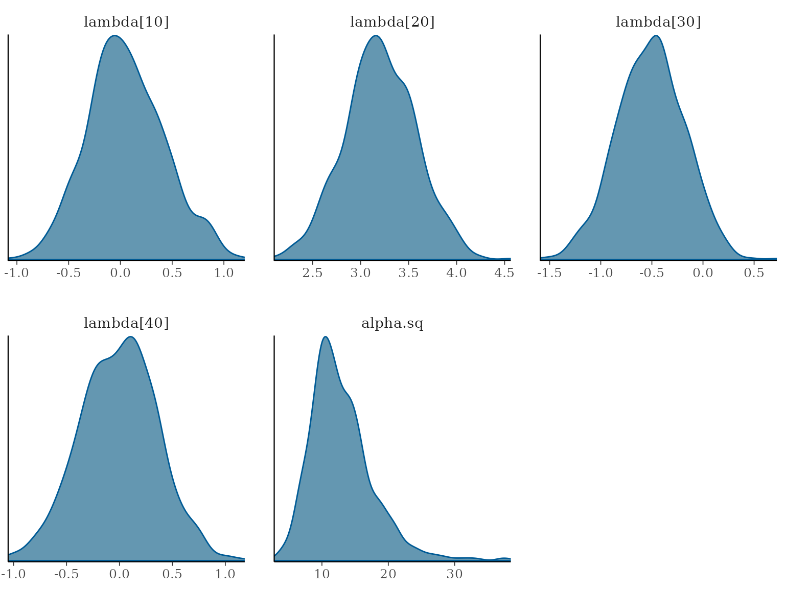
You can use the plot function in coda or
install bayesplot and ggplot2 to get
additional, colourful plots. For example, you can use the
mcmc_intervals() function to create interval plots of the
parameter posterior distributions and the mcmc_dens()
function to create density plots of the MCMC samples. For more
information, see the bayesplot package
documentation.
if (requireNamespace("bayesplot", quietly = TRUE)) {
  # Install bayesplot if not already installed
  # install.packages("bayesplot")
  # install.packages("ggplot2")
  library(bayesplot)
  library(ggplot2)
  # Trace plots
  bayesplot::mcmc_intervals(forcedMarriageModel, pars = c("lambda[10]", "lambda[20]", "lambda[30]", "lambda[40]")) +
    ggtitle("Posterior distributions with 95% credible intervals") +
    ylab(expression(lambda[i])) +
    xlab("Density")
  # Density plots
  bayesplot::mcmc_dens(forcedMarriageModel, pars = c("lambda[10]", "lambda[20]", "lambda[30]", "lambda[40]", "alpha.sq"))
} else {
  # Trace plots
  plot(forcedMarriageModel[, paste0("lambda[", c(10, 20, 30, 40), "]")], main = "Trace plots for item quality parameters")
}